
 English (United Kingdom)
  Italiano (Italia)
CCTV Technologies
In this article I will illustrate how to perform the Optical Calculations for CCTV cameras, others will follow that will address particular conditions to be taken into consideration to optimize the design of a CCTV System.
The following figure illustrates how the vision of an object occurs in the human eye and, similarly, in a camera (or video camera), and introduces the fundamental elements that will be used in the calculations that will follow.
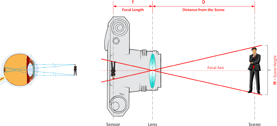
Distance D is also often referred to as "Focal Distance" or "Distance to Scene".
The following figure shows all the optical/geometric parameters involved in the calculations.
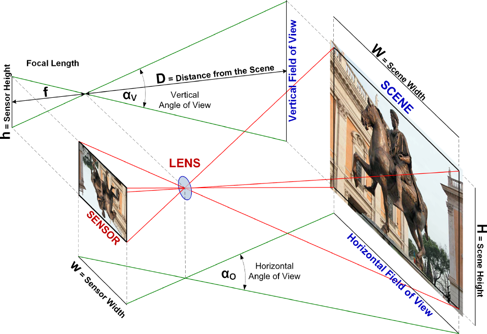
There is a direct proportionality between the size of the sensor and the focal length with respect to the size and distance of the scene:
h/f = H/D – w/f = W/D
from which they are derived:
H = D * h/f – W = D * w/f
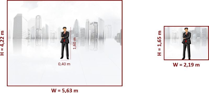
A couple of illustrative examples, both with focusing distance D = 16 m:
- With a 2/3 "sensor, whose dimensions (w x h) are 8.8 x 6.6 mm, and a focal distance f = 25 mm, the dimensions of the scene will be:
H = 16 * 6.6/25 = 4.22 m – W = 16 * 8,8/25 = 5,63 m
- With a 1/3 "sensor, whose dimensions (w x h) are 4.8 x 3.6 mm, and a focal distance f = 35 mm, the scene dimensions will be:
H = 16 * 3.6/35 = 1.65 m – W = 16 * 4,8/35 = 2,19 m
These values correspond to:
If we repeat the same calculation with both focal distances of 25 mm we obtain:
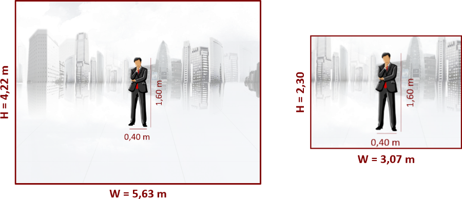
a clear demonstration of the fact that the dimensions of the scenes are directly proportional to those of the sensor used, the greater the size of the latter, the greater the size of the scene being shot.
For the representation of the field of view it is usual to also use the angular representation, which can be schematized as follows:
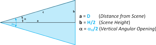
From the 1st Theorem on Right Triangles, we obtain the formulas of the Vertical and Horizontal angles:
aV = 2 * arctg(H/(2 * D)) – aO = 2 * arctg(W/(2 * D))
or, using the previous proportions:
aV = 2 * arctg(h/(2 * f)) – aO = 2 * arctg(w/(2 * f))
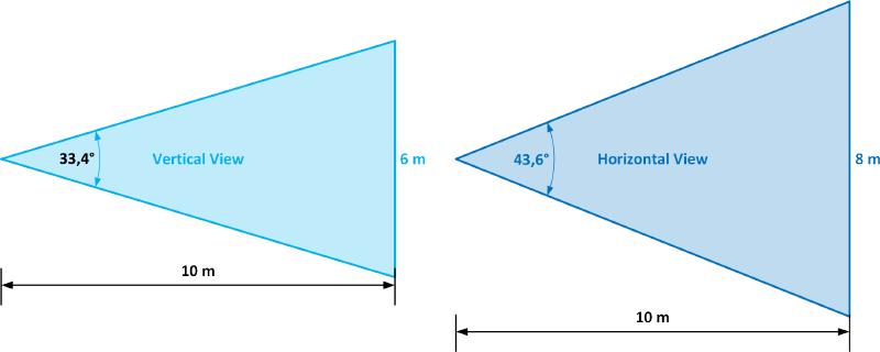
Using a 1/3 "sensor as an example, with a focal distance f = 6 mm and focusing distance D = 10 m, a scene width of 8 x 6 m is obtained, with angles aV = 33.4° and aO = 43.6°.
At this point, assuming that a camera with these parameters is installed at a height of 3 m with a downward inclination of 10°, it is possible to determine the vertical fields of view (dimensions in m):
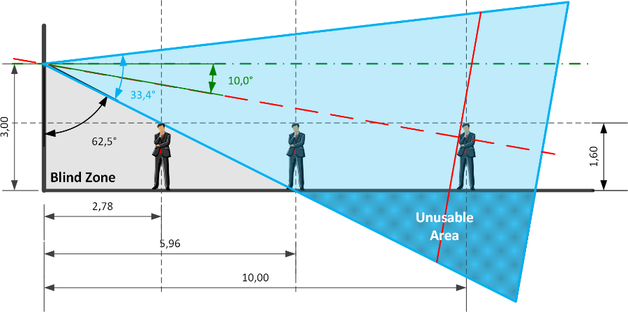
Note the presence of the so-called "Blind Zone", where there is no visual coverage; it depends on the installation height, the angle of inclination and the sensor parameters that determine the angular opening of the shooting field.
In a similar way, it is possible to calculate the horizontal fields of view (top view).
To complete this first article, we will now address the pixel dimensions of the scenes and objects present, which are extremely important in the field of analytics since, in fact, they represent the amount of information available.
Generally, the parameter used is the pixel density, that is the pixels per meter (px/m); for example, in the traditional literature of the sector it is stated that the minimum density required for a face recognition algorithm to work with adequate parameters is 250 px/m (even if this value tends to decrease more and more with the improvement of algorithms based on Artificial Intelligence). So let's see how to calculate these values.
Let's assume we are using a Full HD sensor (1,920 x 1,080 px) with the same parameters as the last example; if the scene width of 8 m corresponds to 1,920 px, the relative horizontal density will be 1,920/8 = 240 px/m, while the vertical one 1,080/6 = 180 px/m.
This difference in values should not arouse astonishment, just think that the sensor dimensions are (generally) in a 4:3 ratio while those in pixels are 16:9; to take this difference into account, a parameter called Pixel Pitch is used which, in some way, takes into account the horizontal and vertical spacing of the sensitive cells (pixels) on the sensor surface. This parameter represents the distance between the centers of 2 adjacent pixels, in practice a mix between the spacing and the dimensions of the pixels, where the spacing can be different for the horizontal and vertical sides.
A clarifying example, suppose we are shooting an object that has 400 x 400 real pixels, for example a circle with a radius of 200 px; if the shooting is carried out with a camera placed at 16 m with a focal length of 25 mm, leaving out the formulas, the horizontal and vertical dimensions will be:
- 50 and 55 for a sensor with a resolution of 704 x 576
- 136 and 102 for a sensor with 1,920 x 1,080 resolution
Strange, right? In practice we frame a perfect circle but on the sensor we get respectively:

This phenomenon must be taken into due consideration when performing geometric calculations in the context of scene analysis.
Finally, we calculate the pixel dimensions of an object (of known size) in a scene. The calculations are performed simply by applying the proportions between the dimensions of the scene and those of the object; for example, in the previous 4.22 x 5.63 m scene with a Full HD sensor the pixels of the person are:
pxV = 1,080 * 1.6/4.22 = 409 – pxO = 1,920 * 0.4/5.63 = 136
while for the other scene of 2.30 x 3.07 m:
pxV = 1,080 * 1.6/2.30 = 752 – pxO = 1,920 * 0.4/3.07 = 250
As proof of the previous phenomenon, we calculate the pixels of a circle with a radius of 1 m, this will be 513 x 682 in the first case and 939 x 1,250 in the second.